states <- as.data.frame(state.x77) |>
rename(life_exp = `Life Exp`, hs_grad = `HS Grad`, murder = Murder)11 Multiple regression
11.1 The multiple regression model
We want to model life_exp as a function of hs_grad and murder (the murder rate per 100,000 population in 1976). We can write the equation this way:
\[\text{LIFEEXP}_i = \beta_0 + \beta_1(\text{HSGRAD}_i) + \beta_2(\text{MURDER}_i) + \varepsilon_i\]
Or we could write it in the more general notation we saw in Chapter 9:
\[\begin{align} \text{LIFEEXP}_i &\sim \mathcal{N}(\mu_i, \sigma) \\ \mu_i &= \beta_0 + \beta_1(\text{HSGRAD}_i) + \beta_2(\text{MURDER}_i) \end{align}\]
Before estimating the model, here’s a quick visualization of the three variables. You can see that all of them are correlated with each other. That is, there is at least some redundancy among the predictors.
Show code
# clear theme because pairs() doesn't work with the changes it makes to par()
tinytheme()

# pairs plot
states |>
  select(life_exp, hs_grad, murder) |>
  pairs()

# reset the theme
tinytheme("ipsum",
          family = book_font,
          palette.qualitative = "Tableau 10",
          palette.sequential = "agSunset")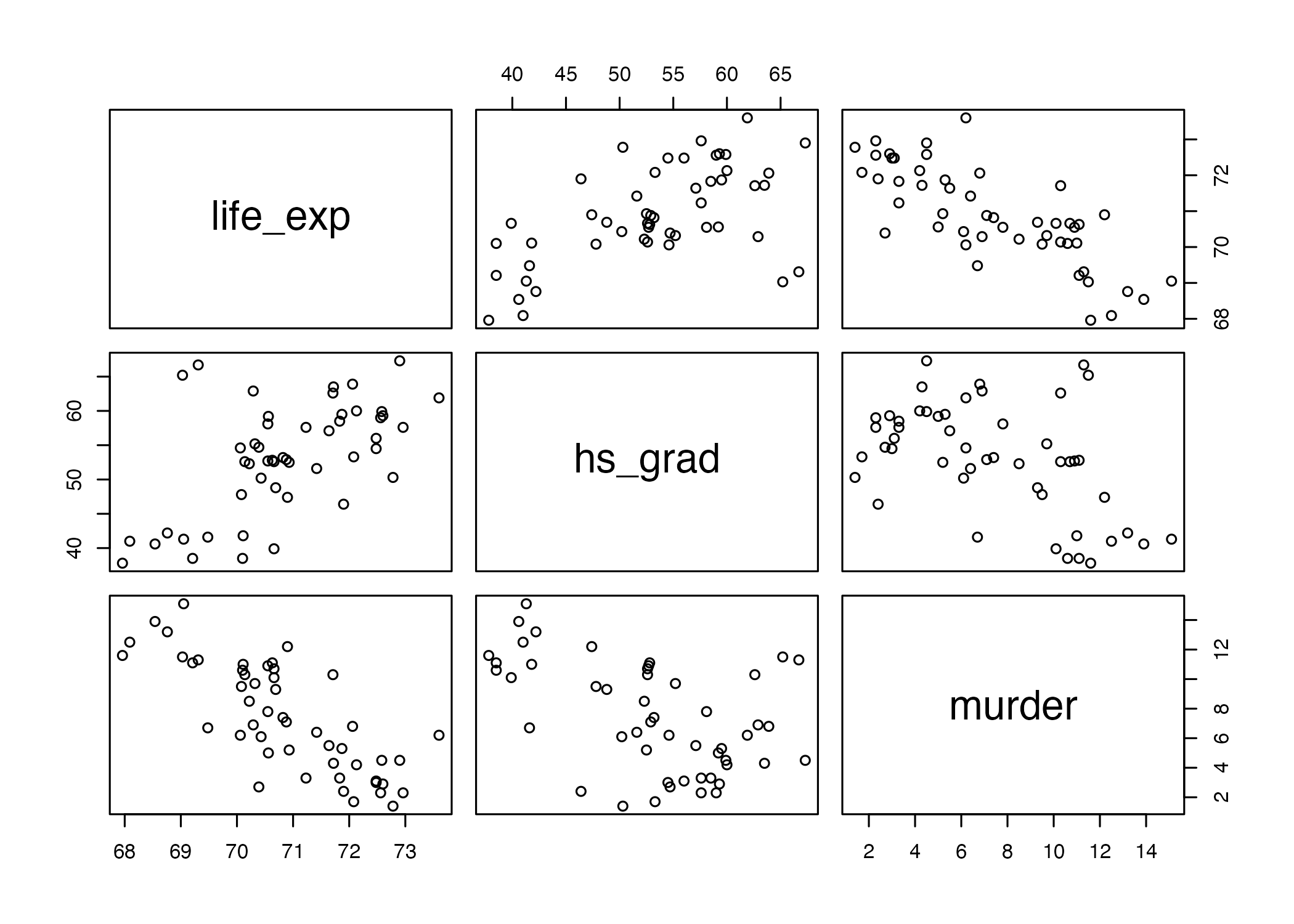
We can quantify this using a correlation matrix.
round(cor(states[, c("life_exp", "hs_grad", "murder")]), 3) life_exp hs_grad murder
life_exp 1.000 0.582 -0.781
hs_grad 0.582 1.000 -0.488
murder -0.781 -0.488 1.000These are the Pearson’s \(r\) correlations. What would the PREs/\(R^2\)s be for the separate simple regressions of life expectancy on these predictors?
simple_hs     <- lm(life_exp ~ hs_grad, data = states)
simple_murder <- lm(life_exp ~ murder,  data = states)

c(hs_grad = summary(simple_hs)$r.squared,
  murder  = summary(simple_murder)$r.squared)
hs_grad murder
0.3389757 0.6097201 11.2 Estimating parameters in multiple regression
Let’s estimate the two-predictor model.
fit <- lm(life_exp ~ hs_grad + murder, data = states)

msummary(fit, gof_map = c("nobs", "r.squared", "rmse"))| (1) | |
|---|---|
| (Intercept) | 70.297 |
| (1.016) | |
| hs_grad | 0.044 |
| (0.016) | |
| murder | -0.237 |
| (0.035) | |
| Num.Obs. | 50 |
| R2 | 0.663 |
| RMSE | 0.77 |
Now here’s a plot. The red points are positive residuals and the blue points are negative residuals.1
1 I got this from ChatGPT 5.2 and made just a few tweaks. I never make these so I really had no idea where to start…
Show code
df <- model.frame(fit)
x  <- df$hs_grad
y  <- df$murder
z  <- df$life_exp
zh <- fitted(fit)

# colors
blue_a <- rgb(0, 0, 1, alpha = 0.35)
red_a  <- rgb(1, 0, 0, alpha = 1)

# color by residual sign: red = above plane, blue = below plane
res  <- z - zh
cols <- ifelse(res > 0, red_a, ifelse(res < 0, blue_a, "gray40"))

# prediction grid for the plane
gx <- seq(min(x), max(x), length.out = 40)
gy <- seq(min(y), max(y), length.out = 40)
grid <- expand.grid(hs_grad = gx, murder = gy)
Z <- matrix(predict(fit, newdata = grid), nrow = length(gx), ncol = length(gy))

# padding
zlim <- range(c(z, Z), na.rm = TRUE)
pad  <- diff(zlim) * 0.05
zlim <- zlim + c(-pad, pad)

# graph
pmat <- persp(
  x = gx, y = gy, z = Z,
  theta = 120, phi = 15,
  zlim = zlim,
  xlab = "HS grad %", ylab = "Murder rate", zlab = "Life expectancy",
  ticktype = "detailed"
)

# projected points and "sticks"
p_obs <- trans3d(x, y, z,  pmat = pmat)
p_fit <- trans3d(x, y, zh, pmat = pmat)
segments(p_fit$x, p_fit$y, p_obs$x, p_obs$y, col = cols, lwd = 1)
points(p_obs, pch = 16, cex = 0.8, col = cols)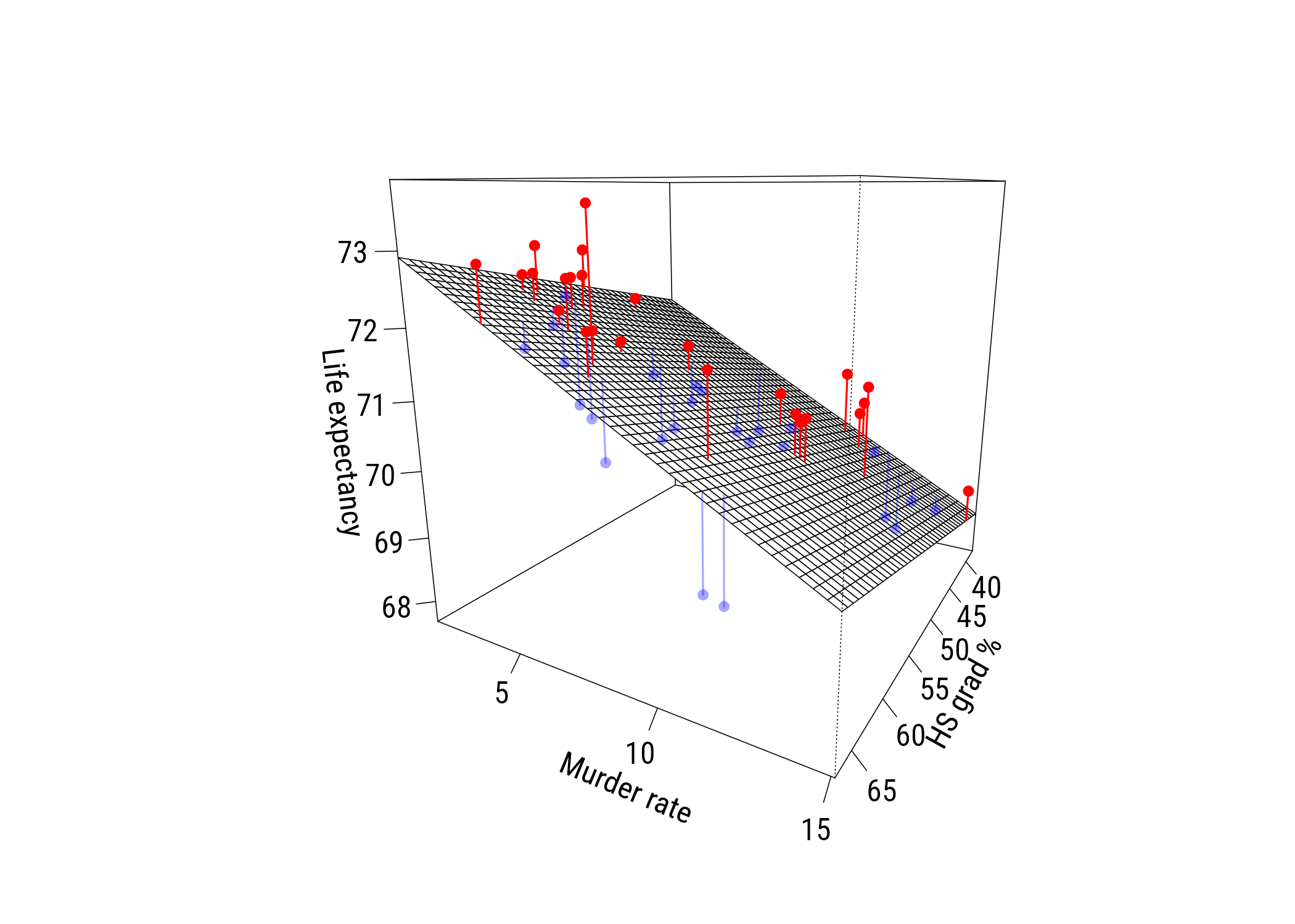
Notice that the coefficient for graduation rate changed. On its own, it was 0.0968. Adjusting for the murder rate, it’s 0.0439 (less than half as big).
11.3 Interpreting parameters in multiple regression
11.3.1 Getting the language right
Here is how I might interpret these coefficients:
According to the model, adjusting for the murder rate, each additional percentage point of high school graduation predicts .044 more years of life expectancy.
According to the model, adjusting for the high school graduation rate, each unit increase in the murder rate per 100,000 predicts .237 fewer years of life expectancy.
A couple of important things are:
- use “adjusting” rather than controlling (the language is, appropriately, weaker)
- avoid causal language and focus on “expectation” and “prediction” conditional on your specific model
WarningAdjusting for a variable is not the same as removing its influence
It’s tempting to read “adjusting for the murder rate” as “as if murder rates were equal everywhere.” But that’s not quite what the model does. It removes the part of graduation rates that’s linearly related to murder rates in these data, and that’s all. It doesn’t adjust for anything we didn’t measure.
11.3.2 Comparing coefficients
These predictors are on different units. HS graduation is percentages and the murder rate is per 100,000. But it’s also worth pointing out that graduating from high school is (fortunately) more common than being murdered. How could we compare the sizes of these coefficients?
Here are the results with x-normalization.
normalized_x <- states |>
  mutate(hs_grad01 = scales::rescale(hs_grad),
         murder01 = scales::rescale(murder))

coef(lm(life_exp ~ hs_grad01 + murder01, data = normalized_x))
(Intercept) hs_grad01 murder01
71.624098 1.294675 -3.248134 How would you interpret these? Be sure to use the correct units!
Here are the results with x-standardization. Interpret these. Be sure to use the correct units!
standardized_x <- states |>
  mutate(hs_z = as.numeric(scale(hs_grad)),
         murder_z = as.numeric(scale(murder)))

coef(lm(life_exp ~ hs_z + murder_z, data = standardized_x))
(Intercept) hs_z murder_z
70.8786000 0.3544776 -0.8752275 Here are the results with full standardization.
fully <- standardized_x |>
  mutate(life_z = as.numeric(scale(life_exp)))

coef(lm(life_z ~ hs_z + murder_z, data = fully))
(Intercept) hs_z murder_z
-3.514457e-15 2.640639e-01 -6.519902e-01 These can be considered partial correlations as well as partial regression coefficients.
11.4 More intuition
How does multiple regression work? We can build a two-predictor multiple regression out of a series of simple regressions.2
2 This is sometimes referred to as the Frisch-Waugh-Lovell theorem but it looks like first credit for this goes to Udny Yule in 1907.
Here it is for hs_grad:
hs_resid   <- residuals(lm(hs_grad  ~ murder, data = states))
life_resid <- residuals(lm(life_exp ~ murder, data = states))

coef(lm(life_resid ~ hs_resid))[2]
hs_resid
0.0438873 You can confirm this is the same as \(b_1\) for hs_grad estimated above.
Now for murder:
murder_resid <- residuals(lm(murder   ~ hs_grad, data = states))
life_resid2  <- residuals(lm(life_exp ~ hs_grad, data = states))

coef(lm(life_resid2 ~ murder_resid))[2]
murder_resid
-0.2370901 You can confirm this is the same as \(b_2\) for murder estimated above.
c(b1 = unname(coef(fit)[2]), b2 = unname(coef(fit)[3])) b1 b2
0.0438873 -0.2370901 This two-step procedure should give you some sense of what we mean when we talk about “adjustment”; we are pulling the influence of a third variable3 out of the relationship with the other two and then estimating a “simple” regression on those adjusted variables.
3 We’re usually (as in this case) “pulling it out” under the assumption that the relationships between that third variable and the other two are linear.
plt(life_resid ~ hs_resid, type = "p",
    xlab = "Graduation rate (murder rate removed)",
    ylab = "Life expectancy (murder rate removed)")

abline(lm(life_resid ~ hs_resid), lwd = 2)
ggplot(data.frame(hs_resid, life_resid), aes(x = hs_resid, y = life_resid)) +
  geom_point() +
  geom_smooth(method = "lm", se = FALSE, color = "black") +
  labs(x = "Graduation rate (murder rate removed)",
       y = "Life expectancy (murder rate removed)")
`geom_smooth()` using formula = 'y ~ x'
11.5 Statistical inference in multiple regression
There’s not much to add here conceptually beyond what we did for simple regression. But I’ll add a couple of things.
confint(fit) 2.5 % 97.5 %
(Intercept) 68.25382379 72.34034424
hs_grad 0.01144419 0.07633041
murder -0.30807483 -0.16610536Neither interval includes zero. We can also still compare models. For example, is it worth adding graduation rate to a model that already has the murder rate?
anova(simple_murder, fit)Analysis of Variance Table
Model 1: life_exp ~ murder
Model 2: life_exp ~ hs_grad + murder
Res.Df RSS Df Sum of Sq F Pr(>F)
1 48 34.461
2 47 29.770 1 4.691 7.4059 0.009088 **
---
Signif. codes: 0 '***' 0.001 '**' 0.01 '*' 0.05 '.' 0.1 ' ' 1pre <- (deviance(simple_murder) - deviance(fit)) / deviance(simple_murder)
pre[1] 0.136122811.5.1 Bootstrapping
We can use bootstrapping to demonstrate how sample size and sampling variability affect the precision of our parameter estimates.
set.seed(522)

# get function that spits out estimates
get_parameter_estimates <- function(formula, data) {

  ## estimate model
  fit <- lm(formula = formula, data = data)

  ## extract and name sigma
  s <- sigma(fit)
  names(s) <- "sigma"

  ## put together all params
  params <- c(coef(fit), s)

  ## return them
  return(params)

}

# create skeleton and iterate with resampling
myboots <- tibble(sim_id = 1:1000) |>
  rowwise() |>
  mutate(params = list(get_parameter_estimates(
    formula = life_exp ~ hs_grad + murder,
    data = slice_sample(states,
                        n = 50,
                        replace = TRUE)))) |>
  unnest_longer(params,
                values_to = "value",
                indices_to = "term")
This is the data structure we have.
print(myboots, n = 8)# A tibble: 4,000 x 3
sim_id term value
<int> <chr> <dbl>
1 1 (Intercept) 71.1
2 1 hs_grad 0.0320
3 1 murder -0.259
4 1 sigma 0.778
5 2 (Intercept) 70.1
6 2 hs_grad 0.0483
7 2 murder -0.236
8 2 sigma 0.811
# i 3,992 more rowsWe can plot the four parameters using density plots.
plt(~ value,
    data = myboots,
    main = "Bootstrap estimates",
    sub = "1000 samples",
    facet = term,
    facet.args = list(free = TRUE),
    type = type_density(joint.bw = "none"),
    yaxt = "n",
    ylab = "",
    xlab = "",
    lw = 2)
ggplot(myboots, aes(x = value)) +
  geom_density(linewidth = 1, color = tableau10[1]) +
  facet_wrap(~term, scales = "free") +
  labs(
    title = "Bootstrap estimates",
    subtitle = "1000 samples",
    x = NULL, y = NULL) +
  theme(axis.text.y = element_blank(), axis.ticks.y = element_blank())
This shows the uncertainty in the estimates across the bootstrap samples.
11.5.2 When predictors overlap
When two predictors are highly correlated, there isn’t much unique variation left in either one to estimate its coefficient. We can see this with a simulation:
set.seed(522)

get_se <- function(rho, n = 400) {

  d <- tibble(
    x1 = rnorm(n),
    x2 = rho * x1 + sqrt(1 - rho^2) * rnorm(n)
  ) |>
    mutate(y = 0.5 * x1 + 0.5 * x2 + rnorm(n))

  fit <- lm(y ~ x1 + x2, data = d)

  coef(summary(fit))["x1", "Std. Error"]

}

expand_grid(
  rep = 1:400,
  rho = c(0, 0.3, 0.6, 0.9, 0.95)
) |>
  rowwise() |>
  mutate(se = get_se(rho)) |>
  group_by(rho) |>
  summarize(mean_SE = round(mean(se), 4), .groups = "drop")
# A tibble: 5 x 2
rho mean_SE
<dbl> <dbl>
1 0 0.0502
2 0.3 0.0526
3 0.6 0.0626
4 0.9 0.115
5 0.95 0.160 The true coefficient is .5 in every one of these simulations, but the standard error gets bigger as the correlation between the predictors goes up. This is called collinearity. It doesn’t bias the estimates, but it makes them less precise.
11.6 Recap
- multiple regression predicts an outcome from two or more predictors at once
- correlated predictors mean redundancy, and coefficients change when predictors are added or removed
- a coefficient is the slope on the part of that predictor not explained by the others
- you can build it out of simple regressions (Frisch-Waugh-Lovell)
- write “adjusting for,” not “controlling for,” and attribute conclusions to the model
- fully standardized coefficients are partial correlations
- collinearity inflates standard errors without biasing estimates