pacman::p_load(dplyr,
               tidyr,
               broom,
               stringr,
               emmeans,
               modelsummary,
               marginaleffects,
               ggeffects,
               tinyplot,
ggplot2)Chapter 11
NOTHING HERE REALLY YET
Goals
To finish the ANOVA/ANCOVA section with our dignity intact.
Set up
tinytheme("ipsum",
          family = "Roboto Condensed",
          palette.qualitative = "Tableau 10",
          palette.sequential = "agSunset")
# Match tinyplot ipsum style
theme_set(
theme_minimal(base_family = "Roboto Condensed") +
theme(panel.grid.minor = element_blank())
)
# Match Tableau 10 palette used by tinytheme (hex codes from ggthemes)
tableau10 <- c("#5778a4", "#e49444", "#d1615d", "#85b6b2", "#6a9f58",
"#e7ca60", "#a87c9f", "#f1a2a9", "#967662", "#b8b0ac")
options(
ggplot2.discrete.colour = \() scale_color_manual(values = tableau10),
ggplot2.discrete.fill = \() scale_fill_manual(values = tableau10)
)gss <- readRDS("data/gss2024.rds") |>
select(id, tvhours, sex, degree, age) |>
drop_na() |>
haven::zap_labels()m1 <- lm(tvhours ~ poly(age, 5) * factor(sex),
data = gss)
summary(m1)
Call:
lm(formula = tvhours ~ poly(age, 5) * factor(sex), data = gss)

Residuals:
    Min      1Q  Median      3Q     Max
-5.5857 -1.7370 -0.7111  0.7383 21.3271

Coefficients:
                           Estimate Std. Error t value Pr(>|t|)
(Intercept)                  3.2063     0.1074  29.865  < 2e-16 ***
poly(age, 5)1               32.5273     4.8049   6.770 1.67e-11 ***
poly(age, 5)2                9.3945     4.9895   1.883   0.0599 .
poly(age, 5)3               -8.8778     5.0950  -1.742   0.0816 .
poly(age, 5)4               -5.7797     5.1326  -1.126   0.2603
poly(age, 5)5               12.3663     4.9872   2.480   0.0132 *
factor(sex)2                 0.1949     0.1432   1.361   0.1737
poly(age, 5)1:factor(sex)2  -5.5344     6.5316  -0.847   0.3969
poly(age, 5)2:factor(sex)2   7.1800     6.5927   1.089   0.2762
poly(age, 5)3:factor(sex)2   2.2800     6.6310   0.344   0.7310
poly(age, 5)4:factor(sex)2   6.4230     6.6633   0.964   0.3352
poly(age, 5)5:factor(sex)2  -0.3673     6.6066  -0.056   0.9557
---
Signif. codes:  0 '***' 0.001 '**' 0.01 '*' 0.05 '.' 0.1 ' ' 1

Residual standard error: 3.235 on 2074 degrees of freedom
Multiple R-squared:  0.05789,   Adjusted R-squared:  0.05289
F-statistic: 11.58 on 11 and 2074 DF, p-value: < 2.2e-16ggpredict(m1, terms = c("age", "sex")) |> plot()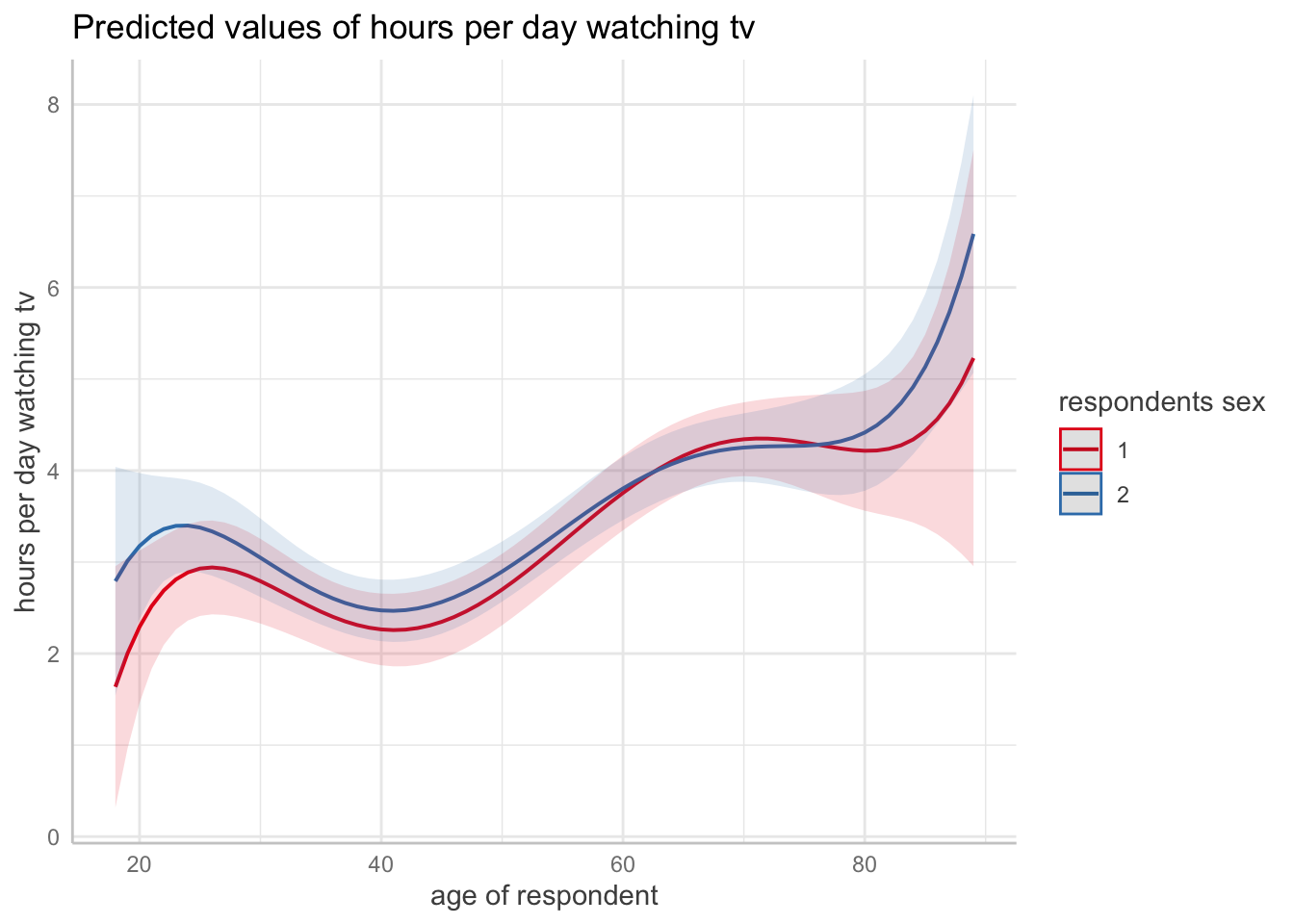
checkpoly <- function(n) {

  tmp <- lm(tvhours ~ poly(age, n) * factor(sex),
         data = gss)

  glance(tmp)[1,8]

}
Let’s look at an experiment.
d <- readRDS("data/lalonde_exp.rds") |>
  mutate(treat_fac = factor(treat,
labels = c("control", "treat")))plt(re78 ~ treat_fac,
data = d,
type = "box")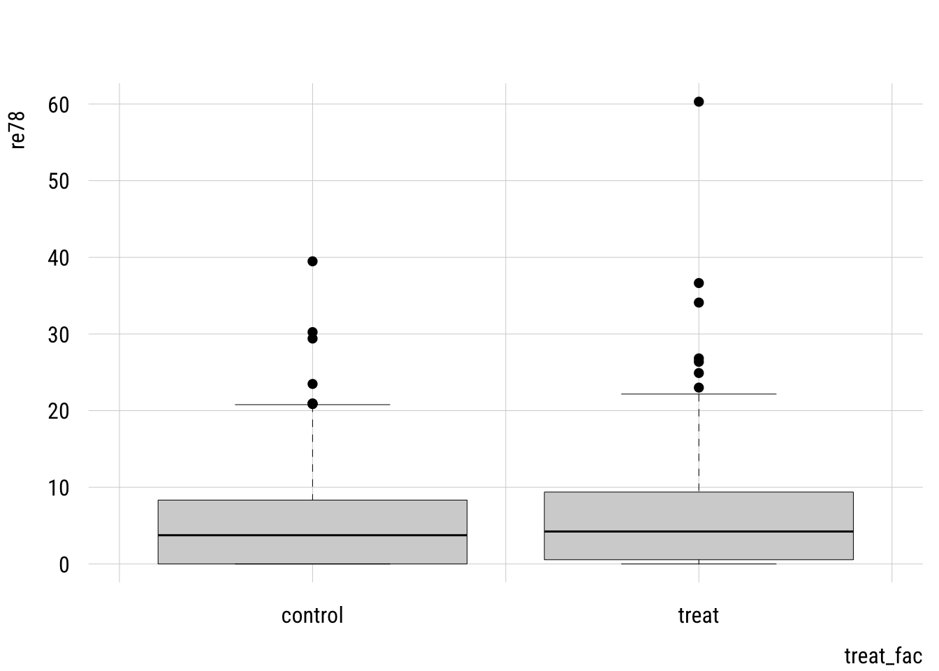
plt(re78 ~ treat_fac,
    data = d,
    type = type_jitter(factor = .5))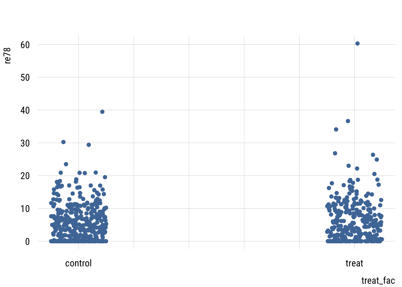
m1 <- lm(re78 ~ treat_fac,
         data = d)
summary(m1)
Call:
lm(formula = re78 ~ treat_fac, data = d)

Residuals:
   Min     1Q Median     3Q    Max
-5.976 -5.090 -1.519  3.361 54.332

Coefficients:
               Estimate Std. Error t value Pr(>|t|)
(Intercept)      5.0900     0.3028  16.811   <2e-16 ***
treat_factreat   0.8863     0.4721   1.877   0.0609 .
---
Signif. codes:  0 '***' 0.001 '**' 0.01 '*' 0.05 '.' 0.1 ' ' 1

Residual standard error: 6.242 on 720 degrees of freedom
Multiple R-squared:  0.004872,  Adjusted R-squared:  0.003489
F-statistic: 3.525 on 1 and 720 DF,  p-value: 0.06086
m2 <- lm(re78 ~ treat_fac + re75,
data = d)
summary(m2)
Call:
lm(formula = re78 ~ treat_fac + re75, data = d)

Residuals:
    Min      1Q  Median      3Q     Max
-10.188  -4.512  -1.498   3.104  54.672

Coefficients:
               Estimate Std. Error t value Pr(>|t|)
(Intercept)     4.51238    0.32932  13.702  < 2e-16 ***
treat_factreat  0.87878    0.46671   1.883   0.0601 .
re75            0.19086    0.04536   4.207 2.91e-05 ***
---
Signif. codes:  0 '***' 0.001 '**' 0.01 '*' 0.05 '.' 0.1 ' ' 1

Residual standard error: 6.171 on 719 degrees of freedom
Multiple R-squared:  0.02878,   Adjusted R-squared:  0.02608
F-statistic: 10.65 on 2 and 719 DF,  p-value: 2.756e-05
m_diff <- lm(I(re78 - re75) ~ treat_fac,
data = d)
summary(m_diff)
Call:
lm(formula = I(re78 - re75) ~ treat_fac, data = d)

Residuals:
    Min      1Q  Median      3Q     Max
-37.995  -3.198  -1.442   3.677  56.114

Coefficients:
               Estimate Std. Error t value Pr(>|t|)
(Intercept)      2.0634     0.3593   5.743 1.37e-08 ***
treat_factreat   0.8469     0.5601   1.512    0.131
---
Signif. codes:  0 '***' 0.001 '**' 0.01 '*' 0.05 '.' 0.1 ' ' 1

Residual standard error: 7.406 on 720 degrees of freedom
Multiple R-squared:  0.003165,  Adjusted R-squared:  0.00178
F-statistic: 2.286 on 1 and 720 DF,  p-value: 0.131
m2_constrained <- lm(re78 ~ treat_fac,
offset = re75,
data = d)
summary(m2_constrained)
Call:
lm(formula = re78 ~ treat_fac, data = d, offset = re75)

Residuals:
    Min      1Q  Median      3Q     Max
-37.995  -3.198  -1.442   3.677  56.114

Coefficients:
               Estimate Std. Error t value Pr(>|t|)
(Intercept)      2.0634     0.3593   5.743 1.37e-08 ***
treat_factreat   0.8469     0.5601   1.512    0.131
---
Signif. codes:  0 '***' 0.001 '**' 0.01 '*' 0.05 '.' 0.1 ' ' 1

Residual standard error: 7.406 on 720 degrees of freedom
Multiple R-squared:  0.003165,  Adjusted R-squared:  0.00178
F-statistic: 2.286 on 1 and 720 DF,  p-value: 0.131
m3 <- lm(re78 ~ treat_fac + re75 + re74 + age + educ +
black + hisp + nodegr + u74 + u75 + married,
data = d)
summary(m3)
Call:
lm(formula = re78 ~ treat_fac + re75 + re74 + age + educ + black +
    hisp + nodegr + u74 + u75 + married, data = d)

Residuals:
    Min      1Q  Median      3Q     Max
-10.395  -4.431  -1.455   3.189  53.911

Coefficients:
               Estimate Std. Error t value Pr(>|t|)
(Intercept)     3.18568    2.63786   1.208   0.2276
treat_factreat  0.82365    0.46846   1.758   0.0791 .
re75            0.06472    0.09145   0.708   0.4794
re74            0.12741    0.07526   1.693   0.0909 .
age             0.01024    0.03707   0.276   0.7824
educ            0.20059    0.18052   1.111   0.2669
black          -1.41919    0.80195  -1.770   0.0772 .
hisp            0.29929    1.05046   0.285   0.7758
nodegr         -0.29961    0.74798  -0.401   0.6889
u74             1.52993    0.93782   1.631   0.1033
u75            -1.00584    0.91702  -1.097   0.2731
married         0.04854    0.65220   0.074   0.9407
---
Signif. codes:  0 '***' 0.001 '**' 0.01 '*' 0.05 '.' 0.1 ' ' 1

Residual standard error: 6.147 on 710 degrees of freedom
Multiple R-squared:  0.04827,   Adjusted R-squared:  0.03353
F-statistic: 3.274 on 11 and 710 DF,  p-value: 0.0002169
m4 <- lm(re78 ~ treat + re75 + I(re75^2) + re74 + I(re74^2)
+ age + I(age^2) + educ + I(educ^2) + black + hisp + married
+ nodegr + u74 + u75,
data = d)
summary(m4)
Call:
lm(formula = re78 ~ treat + re75 + I(re75^2) + re74 + I(re74^2) +
    age + I(age^2) + educ + I(educ^2) + black + hisp + married +
    nodegr + u74 + u75, data = d)

Residuals:
    Min      1Q  Median      3Q     Max
-11.465  -4.435  -1.491   3.296  53.923

Coefficients:
             Estimate Std. Error t value Pr(>|t|)
(Intercept) 10.985771   5.330026   2.061   0.0397 *
treat        0.813809   0.468155   1.738   0.0826 .
re75         0.181010   0.193615   0.935   0.3502
I(re75^2)   -0.003420   0.006532  -0.524   0.6007
re74        -0.182819   0.180101  -1.015   0.3104
I(re74^2)    0.010120   0.005322   1.902   0.0576 .
age         -0.134437   0.216422  -0.621   0.5347
I(age^2)     0.002486   0.003606   0.689   0.4909
educ        -1.181805   1.014489  -1.165   0.2444
I(educ^2)    0.079069   0.055673   1.420   0.1560
black       -1.418940   0.800419  -1.773   0.0767 .
hisp         0.265324   1.049633   0.253   0.8005
married      0.152768   0.654873   0.233   0.8156
nodegr       0.312865   0.910017   0.344   0.7311
u74          0.712339   1.036152   0.687   0.4920
u75         -0.947228   0.968743  -0.978   0.3285
---
Signif. codes:  0 '***' 0.001 '**' 0.01 '*' 0.05 '.' 0.1 ' ' 1

Residual standard error: 6.132 on 706 degrees of freedom
Multiple R-squared:  0.05846,   Adjusted R-squared:  0.03846
F-statistic: 2.922 on 15 and 706 DF,  p-value: 0.0001621
m5 <- lm(re78 ~ treat * (re75 + re74 + age + educ + nodegr +
black + hisp + married),
data = d)
summary(m5)
Call:
lm(formula = re78 ~ treat * (re75 + re74 + age + educ + nodegr +
    black + hisp + married), data = d)

Residuals:
    Min      1Q  Median      3Q     Max
-11.444  -4.335  -1.603   3.298  54.374

Coefficients:
               Estimate Std. Error t value Pr(>|t|)
(Intercept)    6.517070   3.437699   1.896   0.0584 .
treat         -6.551504   5.241558  -1.250   0.2117
re75           0.210366   0.112566   1.869   0.0621 .
re74           0.068945   0.088207   0.782   0.4347
age           -0.011283   0.046925  -0.240   0.8101
educ          -0.015309   0.242965  -0.063   0.9498
nodegr        -0.632323   1.004967  -0.629   0.5294
black         -1.589615   1.084345  -1.466   0.1431
hisp           0.539836   1.371852   0.394   0.6941
married       -1.012499   0.857109  -1.181   0.2379
treat:re75    -0.261151   0.181527  -1.439   0.1507
treat:re74     0.000318   0.149470   0.002   0.9983
treat:age      0.057136   0.073886   0.773   0.4396
treat:educ     0.517990   0.361004   1.435   0.1518
treat:nodegr   0.852859   1.502433   0.568   0.5705
treat:black    0.589770   1.606731   0.367   0.7137
treat:hisp    -0.801334   2.132576  -0.376   0.7072
treat:married  2.418215   1.320962   1.831   0.0676 .
---
Signif. codes:  0 '***' 0.001 '**' 0.01 '*' 0.05 '.' 0.1 ' ' 1

Residual standard error: 6.123 on 704 degrees of freedom
Multiple R-squared:  0.06363,   Adjusted R-squared:  0.04101
F-statistic: 2.814 on 17 and 704 DF, p-value: 0.0001321avg_slopes(m5, variables = "treat")
 Estimate Std. Error    z Pr(>|z|)   S   2.5 % 97.5 %
    0.819      0.466 1.76    0.079 3.7 -0.0947   1.73

Term: treat
Type: response
Comparison: 1 - 0
m1 <- glm(tvhours ~ age,
data = gss,
family = poisson())
summary(m1)
Call:
glm(formula = tvhours ~ age, family = poisson(), data = gss)

Coefficients:
             Estimate Std. Error z value Pr(>|z|)
(Intercept) 0.6199166  0.0385197   16.09   <2e-16 ***
age         0.0111123  0.0006796   16.35   <2e-16 ***
---
Signif. codes:  0 '***' 0.001 '**' 0.01 '*' 0.05 '.' 0.1 ' ' 1

(Dispersion parameter for poisson family taken to be 1)

    Null deviance: 5366.4  on 2085  degrees of freedom
Residual deviance: 5098.1  on 2084  degrees of freedom
AIC: 10657

Number of Fisher Scoring iterations: 5ggpredict(m1, terms = "age") |> plot()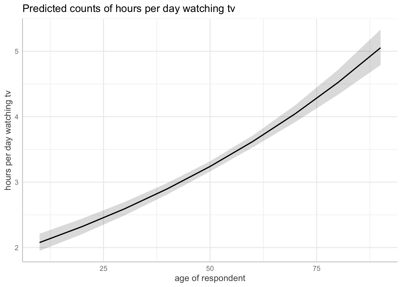
d <- d |>
  mutate(re78 = floor(re78 * 1000),
         re75 = floor(re75 * 1000),
         re74 = floor(re74 * 1000))

m1 <- glm(re78 ~ treat_fac,
          data = d,
          family = poisson())
summary(m1)
Call:
glm(formula = re78 ~ treat_fac, family = poisson(), data = d)

Coefficients:
                Estimate Std. Error z value Pr(>|z|)
(Intercept)    8.5349735  0.0006799 12553.4   <2e-16 ***
treat_factreat 0.1605231  0.0010127   158.5   <2e-16 ***
---
Signif. codes:  0 '***' 0.001 '**' 0.01 '*' 0.05 '.' 0.1 ' ' 1

(Dispersion parameter for poisson family taken to be 1)

    Null deviance: 4851711  on 721  degrees of freedom
Residual deviance: 4826748  on 720  degrees of freedom
AIC: 4832200

Number of Fisher Scoring iterations: 5